Detection of Chagas Disease from the ECG: PhysioNet Challenge 2025

Chagas Disease Overview

• Cause & Transmission: Caused by Trypanosoma cruzi, primarily spread by triatomine insects, but also through blood transfusions, organ transplants, and congenital transmission.

• Disease Progression: Two phases—acute (mild/nonspecific symptoms) and chronic (asymptomatic in most, but 30-40% develop severe complications, mainly cardiac). Early antiparasitic treatment is effective, but loses efficacy as the infection progresses.

• Historical Background: Named after Carlos Chagas, who discovered it in 1909. Chronic complications, especially cardiac and digestive issues, typically appear 10 to 30 years post-infection.

• Diagnosis: Detected via blood tests (parasite detection or serological tests for antibodies).

• Cardiac Impact & ECG Role: Chagas cardiomyopathy can cause heart damage, arrhythmias, conduction disorders, and dilated cardiomyopathy. Severe cases may lead to sudden cardiac death, though the indeterminate chronic form lacks ECG abnormalities, making early detection challenging.

About the Challenge

• The George B. Moody PhysioNet Challenge 2025 [1] is a prestigious annual competition focused on advancing physiological and clinical problem-solving.

• This year’s challenge targets Chagas disease, a serious cardiovascular threat prevalent in Central and South America.

• Participants must develop open-source algorithms to detect Chagas disease using standard 12-lead ECGs.

• The goal is to improve screening efficiency, identifying potential cases for confirmatory serological testing while optimizing healthcare resources.

• Inspired by this, our objective is to build a model that can accurately detect Chagas disease using only a short (~10-second) 12-lead ECG recording.

Dataset

• The 2025 PhysioNet Challenge uses the CODE-15% Database [2], which contains 300,000+ 12-lead ECG recordings collected in Brazil (2010–2016).

• Binary Chagas disease labels are included, based on self-reported diagnoses and potentially supplemented by questionnaire responses.

• Each ECG record has a WFDB header file with metadata such as sampling frequency, signal parameters, demographics (if available), and Chagas labels.

• Example: Record 113 contains 12 channels, 400 Hz sampling frequency, and 4096 samples per channel.

wfdb.plot_wfdb(record=wfdb.rdrecord(record, physical=False), figsize=(20, 10), time_units='samples')

ECG features

Feature Extraction & Data Processing

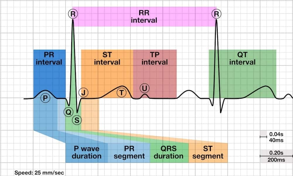
• ECG Feature Extraction: Relevant features are derived from fiducial points (P, Q, R, S, T waves) and segment durations, enabling numerical representation of the ECG signal for machine learning classification.

• Chagas Disease Detection: Research indicates that ECG pattern durations are strongly associated with Chagas disease, making them key diagnostic features.

• Implementation: Feature extraction is handled in preprocessing.py using NeuroKit2 ensuring correct wave order. The extracted features are then merged with the metadata (age, gender, Chagas label) and aggregated in a single csv file.

• Dataset Challenges & Solutions: The dataset is large and imbalanced, making full processing computationally expensive. To mitigate this:

  • A partitioned subset of the data is used for efficient experimentation.
  • Downsampling is applied to balance seropositive and seronegative cases, ensuring unbiased model training.

Exploratory Data Analysis

_, axes = plt.subplots(nrows=8, ncols=6, figsize=(20, 10))
for ax, cname in zip(axes.ravel(), num_cols):
    sn.histplot(data=df, x=cname, bins=50, stat="count", alpha=1, kde=False, multiple='dodge', ax=ax, hue='chagas', legend=False)
plt.tight_layout()
plt.show()

t_test_df.sort_values(by='p_value')

	column	t_stat	p_value	is_significant
6	PR_segment_mean	20.819895	1.633643e-94	True
7	PR_segment_max	20.634896	4.930207e-93	True
5	PR_interval_max	18.113069	2.226532e-72	True
21	HRV_MaxNN	15.886669	2.847833e-56	True
3	PR_interval_mean	15.732206	3.498921e-55	True
0	P_wave_duration_mean	-15.235253	5.901368e-52	True
15	ST_segment_max	14.821371	2.896867e-49	True
17	HRV_SDRMSSD	-14.733790	9.797298e-49	True
19	HRV_Prc80NN	13.986132	4.023160e-44	True
1	P_wave_duration_min	-13.572657	1.116486e-41	True
13	QT_interval_max	12.460313	2.006407e-35	True
22	HRV_HTI	-11.860685	2.772502e-32	True
16	HRV_MedianNN	10.322695	6.949631e-25	True
10	QRS_duration_max	9.578422	1.166052e-21	True
8	QRS_duration_mean	9.532662	1.821155e-21	True
2	P_wave_duration_max	-8.089928	6.502718e-16	True
18	HRV_Prc20NN	6.024534	1.742408e-09	True
4	PR_interval_min	5.904194	3.640283e-09	True
14	ST_segment_mean	5.721862	1.079176e-08	True
12	QT_interval_min	-4.514126	6.416034e-06	True
11	QT_interval_mean	3.694889	2.209494e-04	True
9	QRS_duration_min	3.558609	3.743054e-04	True
20	HRV_MinNN	2.215779	2.672431e-02	True

_, axes = plt.subplots(nrows=1, ncols=2)
for i, cname in enumerate(cat_cols + ['chagas']):
    df[cname].value_counts().plot(kind='bar', ax=axes[i], figsize=figsize, title=cname, ylabel='Count', xlabel='', sharey=True)

plt.tight_layout()

df.groupby('is_male')['chagas'].mean().plot.bar(title='Mean of the target variable conditioned on the gender')
plt.tight_layout()

_, axes = plt.subplots(nrows=8, ncols=6, figsize=(20,10))
for ax, cname in zip(axes.ravel(), num_cols):
    bin_size = (df[cname].max() - df[cname].min()) / 20
    df['chagas'].groupby(df[cname] // bin_size).mean().plot.bar(ax=ax)
plt.tight_layout()

plt.figure(figsize=(27,12))
sn.heatmap(df.corr(method='pearson'), annot=True, vmin=-1, vmax=1, cmap='RdBu')
plt.tight_layout()

A more in-depth analysis of the data

From the literature we see that:

• Strong Link Between Chagas Disease & Abnormal ECG [3]90529-x)

  • Seropositive individuals are 4.3x more likely to show abnormal ECG patterns than seronegative ones.
  • Higher prevalence observed in men.

• Age-Dependent Increase in ECG Abnormalities [3]90529-x)

  • 10-14, ECG abnormalities are similar between the two groups.
  • 25-44, abnormal ECG occurrence is 9.3x higher in seropositive individuals.
  • 44-64, the ratio decreases.
  • 64+, roughly equal proportion between the groups.

How can we recognise an abnormal ecg?

Ventricular Rate

Claim:

• Seropositive persons presents significantly lower ventricular rates [4].

Ventricular Rate: The ventricular rate represents the number of ventricular contractions per minute (beats per minute, BPM) and indicates the heart's electrical pacing.

• A known cause of low Ventricular Rate is the presence of RBBB, that is know to be a symptom of the chagas disease [4]

HRV_MeanNN: MeanNN is the average NN interval (time between normal heartbeats) and is inversely related to ventricular rate.

• Higher MeanNN values indicate a lower ventricular rate

df['age_group'] = pd.qcut(df['age'], q=4)
sn.boxplot(x='age_group', y='HRV_MeanNN', hue='chagas', data=df, showfliers=False, showmeans=True)
plt.tight_layout()
plt.show()

Heart rate variability (HRV_HTI)

Claim:

• Arrhytmias occur 2 times more frequently in seropositive than among seronegative invidivuals [3]90529-x).

HRV_HTI: Measures heart rate regularity, calculated as the total number of RR intervals divided by the height of the RR interval histogram.

• Higher HRV_HTI values indicate more regular RR intervals, while lower values suggest increased irregularity.

sn.boxplot(x='age_group', y='HRV_HTI', hue='chagas', data=df, showfliers=False, showmeans=True)
plt.tight_layout()
plt.show()

ST-T wave abnormalities (ST_slope)

Claim:

• Chagas cardiomyopathy presents nonspecific ST- and T-wave abnormalities [7].
• Common abnormalities are right bundle branch block (RBBB), left anterior fascicular block, and diffuse ST-T changes.

ST_slope: Measures the slope between the S and T wave.

• In RBBB, this manifests as ST depression and/or T-wave inversion.

sn.boxplot(x='age_group', y='ST_slope_mean', hue='chagas', data=df, showfliers=False, showmeans=True)
plt.tight_layout()
plt.show()

QRS Duration

Claim:

• Seropositive people had substantially longer QRS intervals than seronegative persons [3]90529-x) [4].
• 83.5% of individuals with QRS intervals above 0.09s were seropositive, while only 4.4% of seronegative individuals had QRS intervals above this threshold. [3]90529-x)

QRS Duration: is the time between the start of the Q wave and the end of the S wave, representing how long it takes for the ventricles to fully depolarize.

• Prolonged QRS duration may indicate conduction abnormalities linked to Chagas disease.

sn.boxplot(x='age_group', y='QRS_duration_mean', hue='chagas', data=df, showfliers=False, showmeans=True)
plt.tight_layout()
plt.show()

Standardization of the data

The StandardScaler is applied to the numerical columns to have a better distribution of the data by subtracting the mean and dividing by the standard deviation.

We first dropped the age_group column since it was not used inside our models and then applied the StandardScaler to the numerical columns.

The splitting between training and testing sets is done by stratifying the target variable and shuffling the data. For the test set, we used 20% of the data.

X, y = df.drop(columns=['chagas', 'age_group'], axis=1), df['chagas']

X_train, X_test, y_train, y_test = train_test_split(X, y, test_size=0.2, random_state=SEED, stratify=y, shuffle=True)
scaler = StandardScaler()
X_train.iloc[:, :-1] = scaler.fit_transform(X_train.iloc[:, :-1])
X_test.iloc[:, :-1] = scaler.transform(X_test.iloc[:, :-1])

results_dict = {}

def print_results(model, y_test, y_pred, y_pred_proba):
    acc = accuracy_score(y_test, y_pred)
    auc = roc_auc_score(y_test, y_pred_proba)
    f1 = f1_score(y_test, y_pred)
    f_beta = fbeta_score(y_test, y_pred, beta=0.5)
    print(f'Accuracy: {acc:.4f}')
    print(f'ROC-AUC: {auc:.4f}')
    print(f'F1-score: {f1:.4f}')
    print("F-beta score", f_beta)
    cm = confusion_matrix(y_test, y_pred, labels=[0, 1], normalize="all")
    disp = ConfusionMatrixDisplay(confusion_matrix=cm,
                              display_labels=['Seronegative', 'Seropositive'])
    disp.plot()
    plt.show()
    
    return {'acc': acc, 'auc': auc, 'f1': f1, 'f_beta': f_beta}

Logistic Regression

Key Features

• L1 Regularization: Promotes sparsity, identifies less useful features.
• Solver: SAGA chosen for efficiency with L1 and scalability for large datasets.

$$\text{argmin}_{\theta}\ H\biggl(y, f(x,\theta)\biggr) + \frac{1}{C} ||\theta||_1$$

Hyperparameter Tuning

• Parameter C: Controls regularization strength.
• GridSearchCV: Tuned C with ROC-AUC as performance metric.

Insights on Tuning C

• Bias-Variance Tradeoff:
  • Small C → Strong regularization → Risk of underfitting.
  • Large C → Weak regularization → Risk of overfitting.
• Data-Driven Results: Optimal C balances generalization and training performance.
• Benefits of L1: Sparsity, feature selection, improved interpretability.

lr_score_cv, lr_score_test = gscv.best_score_, roc_auc_score(y_test, lr.predict_proba(X_test)[:, 1])
print(f'AUC score for C={lr_params["C"]:.2f}: {lr_score_cv:.2f} (cross-validation), {lr_score_test:.2f} (test)')

AUC score for C=10.00: 0.75 (cross-validation), 0.75 (test)

results_dict['Logistic Regression'] = print_results(lr, y_test, lr.predict(X_test), lr.predict_proba(X_test)[:, 1])

Accuracy: 0.6828
ROC-AUC: 0.7457
F1-score: 0.6722
F-beta score 0.6861796484437994

pd.DataFrame({'variable': X.columns, 'coeff': np.abs(lr.coef_[0]), 'sign': ['neg' if lr.coef_[0][i] < 0 else 'pos' for i in range(len(X.columns))]}).sort_values(by='coeff', ascending=False).head(20)

	variable	coeff	sign
32	HRV_CVNN	0.750192	pos
21	ST_segment_std	0.749812	pos
44	HRV_MaxNN	0.628669	neg
1	P_wave_duration_std	0.615769	pos
22	ST_segment_min	0.547871	pos
3	P_wave_duration_max	0.530417	neg
2	P_wave_duration_min	0.487001	pos
39	HRV_Prc20NN	0.469673	pos
12	QRS_duration_mean	0.452798	pos
20	ST_segment_mean	0.391311	pos
33	HRV_CVSD	0.375549	pos
29	HRV_SDNN	0.357011	pos
16	QT_interval_mean	0.349609	neg
42	HRV_pNN20	0.344252	neg
48	is_male	0.335431	neg
11	PR_segment_max	0.311716	neg
24	ST_slope_mean	0.307068	pos
31	HRV_SDSD	0.277912	neg
43	HRV_MinNN	0.269241	pos
9	PR_segment_std	0.264337	pos

lr_coefs = pd.Series(index=X.columns, data=lr.coef_[0])
lr_coefs.plot(kind='bar', figsize=figsize)
plt.show()

XGBoost

Key Features

• Algorithm: XGBoost with hist tree method for computational efficiency on large datasets.
• Feature Importance:
  • Total Gain Importance: Considers both frequency and magnitude of feature contributions across splits.

Benefits

• Performance: Efficient and effective for large datasets.
• Explainability: Enhances interpretability for AI through detailed feature contribution analysis.

base_est = xgboost.XGBClassifier(tree_method='hist', importance_type='total_gain', n_jobs=-1)
param_grid={'max_depth': [2, 3, 4], 'n_estimators': list(range(20, 41, 5)), 'reg_lambda': np.linspace(0, 500, 6)}
gscv = GridSearchCV(base_est, param_grid=param_grid, n_jobs=-1)
gscv.fit(X_train, y_train)
xbm, xbm_params = gscv.best_estimator_, gscv.best_params_

xbm_score_test = roc_auc_score(y_test, xbm.predict_proba(X_test)[:, 1])
print(f'AUC score for max_depth={xbm_params["max_depth"]}, n_estimators={xbm_params["n_estimators"]}, reg_lambda={xbm_params["reg_lambda"]:.2f}: {xbm_score_test:.2f} (test)')

AUC score for max_depth=4, n_estimators=40, reg_lambda=100.00: 0.78 (test)

results_dict['XGBoost'] = print_results(xbm, y_test, y_pred=xbm.predict(X_test), y_pred_proba=xbm.predict_proba(X_test)[:, 1])

Accuracy: 0.7050
ROC-AUC: 0.7813
F1-score: 0.7145
F-beta score 0.7011177239076789

xbm_imp = pd.Series(index=X.columns, data=xbm.feature_importances_)
xbm_imp.plot(kind='bar', figsize=figsize)
plt.tight_layout()
plt.show()

_, axes = plt.subplots(nrows=2, ncols=3, figsize=(20, 10))
for ax, imp_type in zip(axes.ravel(), ['weight', 'gain', 'cover', 'total_gain', 'total_cover']):
    pd.Series(xbm.get_booster().get_score(importance_type=imp_type)).plot.bar(ax=ax, title=imp_type)
plt.tight_layout()

Permutation Importance

Key Insights

• Data Dependence: Feature importance varies with the dataset.
  • Misconception: Important features are universally best regardless of the dataset.

Methodology

• Definition: Model-agnostic approach.
  • Randomly shuffle feature values.
  • Measure impact on model performance.
• Purpose: Assess feature importance independently of internal model metrics.

Application

• Datasets: Computed on training and testing sets to check consistency.
• Model: Used XGBoost due to its superior performance.

Benefits

• Robust Evaluation: Validates feature importance across models and datasets.
• Model Independence: Avoids reliance on specific model-based metrics.

util.plot_bars(xbm_p_imp, figsize=figsize, std=r_train.importances_std, title='Permutation Feature Importance (train)', rotation=90)

util.plot_bars(xbm_p_imp, figsize=figsize, std=r_test.importances_std, title='Permutation Feature Importance (test)', rotation=90)

SHAP Values

Key Features

• Purpose: Explain predictions of the XGBoost model with high accuracy.
• Origin: Based on Shapley values from game theory.
  • Assigns importance to features by analyzing their marginal contributions across all feature combinations.

Methodology

• Explainer Definition: Created using a sample of 100 training points.
• Computation: SHAP values calculated for the test set.
  • Larger samples improve accuracy but increase computational time (~1 hour for XGBoost).

Comparison

• Versus Permutation Importance:
  • SHAP is more accurate.
  • Provides detailed insights into individual prediction contributions.

Benefits

• Explainability: Highlights the contribution of each feature to model predictions.
• Robustness: Suitable for high-performing models like XGBoost.

f = lambda x: xbm.predict_proba(x)[:,1]
explainer = shap.KernelExplainer(f, shap.sample(X_train, 100), link='logit', seed=SEED)

shap.summary_plot(shap_values, X_test, plot_type='bar', max_display=20)

shap.waterfall_plot(shap.Explanation(values=shap_values[0], base_values=explainer.expected_value, data=X_test.iloc[0], feature_names=X.columns.tolist()), max_display=20)

shap.waterfall_plot(shap.Explanation(values=shap_values[1], base_values=explainer.expected_value, data=X_test.iloc[1], feature_names=X.columns.tolist()), max_display=20)

shap.plots.beeswarm(shap_values, max_display=20)

Feature selection

shap_mean = np.abs(shap_values.values).mean(axis=0)
shap_mean = pd.Series(index=X.columns, data=shap_mean)
shap_mean.sort_values(ascending=False, inplace=True)
best_20_shap = shap_mean.head(20)

X_train_fs = X_train[best_20_shap.index]
X_test_fs = X_test[best_20_shap.index]

base_est = xgboost.XGBClassifier(tree_method='hist', importance_type='total_gain')
param_grid={'max_depth': [2, 3, 4], 'n_estimators': list(range(20, 41, 5)), 'reg_lambda': np.linspace(0, 500, 6)}
gscv_fs = GridSearchCV(base_est, param_grid=param_grid, n_jobs=-1)
gscv_fs.fit(X_train_fs, y_train)
xbm_fs, xbm_params_fs = gscv_fs.best_estimator_, gscv_fs.best_params_
y_pred = xbm_fs.predict_proba(X_test_fs)[:, 1]
xbm_score_test_fs = roc_auc_score(y_test, y_pred)

print(f'AUC score for max_depth={xbm_params_fs["max_depth"]}, n_estimators={xbm_params_fs["n_estimators"]}, reg_lambda={xbm_params_fs["reg_lambda"]:.2f}: {xbm_score_test_fs:.4f} (test)')

AUC score for max_depth=4, n_estimators=40, reg_lambda=100.00: 0.7804 (test)

results_dict['XGBoost-SHAP'] = print_results(xbm_fs, y_test, xbm_fs.predict(X_test_fs), xbm_fs.predict_proba(X_test_fs)[:, 1])

Accuracy: 0.7023
ROC-AUC: 0.7804
F1-score: 0.7103
F-beta score 0.6992238980817104

BorutaPy

• Generate and Evaluate
  1. extend the dataset by adding and shuffling copies of all variables
  2. run a random forest to compute Z-scores for all features
• Compare Scores
  1. finds maximum Z-score among shadow attributes (MZSA)
  2. assign a “hit” to attributes that exceeds this value
• Statistical Testing & Iteration
  1. For undetermined attributes, perform a two-sided test against the MZSA to label them as important or unimportant
  2. remove shadow attributes
  3. repeat until all attributes are classified or limit is reached

bfs = BorutaPy(xbm, n_estimators='auto', max_iter=100, verbose=0, random_state=SEED, early_stopping=True)
bfs.fit(X=X, y=y)

BorutaPy(early_stopping=True,
         estimator=XGBClassifier(base_score=None, booster=None, callbacks=None,
                                 colsample_bylevel=None, colsample_bynode=None,
                                 colsample_bytree=None, device=None,
                                 early_stopping_rounds=None,
                                 enable_categorical=False, eval_metric=None,
                                 feature_types=None, gamma=None,
                                 grow_policy=None, importance_type='total_gain',
                                 interaction_constraints=None,
                                 learning_rate=None, max_bin=None,
                                 max_cat_threshold=None, max_cat_to_onehot=None,
                                 max_delta_step=None, max_depth=4,
                                 max_leaves=None, min_child_weight=None,
                                 missing=nan, monotone_constraints=None,
                                 multi_strategy=None, n_estimators=173,
                                 n_jobs=-1, num_parallel_tree=None,
                                 random_state=381215112, ...),
         n_estimators='auto',
         random_state=RandomState(MT19937) at 0x7682C5A9F340)

In a Jupyter environment, please rerun this cell to show the HTML representation or trust the notebook.
On GitHub, the HTML representation is unable to render, please try loading this page with nbviewer.org.

pd.DataFrame(data=bfs.ranking_, index=X.columns).rename(columns={0: 'Ranking'}).sort_values(by='Ranking', ascending=True)

	Ranking
P_wave_duration_mean	1
ST_segment_mean	1
ST_segment_std	1
ST_segment_min	1
ST_segment_max	1
age	1
ST_slope_min	1
HRV_MeanNN	1
HRV_SDSD	1
HRV_CVNN	1
HRV_CVSD	1
HRV_MCVNN	1
HRV_SDRMSSD	1
HRV_Prc20NN	1
HRV_HTI	1
HRV_TINN	1
QT_interval_max	1
QT_interval_min	1
ST_slope_mean	1
QRS_duration_min	1
QRS_duration_mean	1
PR_segment_mean	1
QT_interval_mean	2
ST_slope_max	2
P_wave_duration_max	3
P_wave_duration_std	4
HRV_Prc80NN	6
HRV_MedianNN	6
is_male	6
PR_segment_std	8
ST_slope_std	9
HRV_pNN20	9
PR_segment_min	11
QT_interval_std	12
HRV_MaxNN	13
PR_interval_min	14
HRV_MinNN	15
QRS_duration_std	16
HRV_IQRNN	16
PR_interval_mean	18
PR_segment_max	18
P_wave_duration_min	20
QRS_duration_max	21
PR_interval_max	22
PR_interval_std	23
HRV_SDNN	24
HRV_pNN50	25
HRV_RMSSD	26
HRV_MadNN	27

X_train_boruta = X_train[X.columns[bfs.ranking_ == 1].values]
X_test_boruta = X_test[X.columns[bfs.ranking_ == 1].values]

base_est = xgboost.XGBClassifier(tree_method='hist', importance_type='total_gain')
param_grid={'max_depth': [2, 3, 4], 'n_estimators': list(range(20, 41, 5)), 'reg_lambda': np.linspace(0, 500, 6)}
gscv_boruta = GridSearchCV(base_est, param_grid=param_grid, n_jobs=-1)
gscv_boruta.fit(X_train_boruta, y_train)
xbm_boruta, xbm_params_boruta = gscv_boruta.best_estimator_, gscv_boruta.best_params_
y_pred = xbm_boruta.predict_proba(X_test_boruta)[:, 1]
xbm_score_test_boruta = roc_auc_score(y_test, y_pred)

print(f'AUC score for max_depth={xbm_params_boruta["max_depth"]}, n_estimators={xbm_params_boruta["n_estimators"]}, reg_lambda={xbm_params_boruta["reg_lambda"]:.2f}: {xbm_score_test_boruta:.4f} (test)')

AUC score for max_depth=4, n_estimators=35, reg_lambda=100.00: 0.7800 (test)

results_dict['XGBoost-Boruta'] = print_results(xbm_boruta, y_test, xbm_boruta.predict(X_test_boruta), xbm_boruta.predict_proba(X_test_boruta)[:, 1])

Accuracy: 0.7081
ROC-AUC: 0.7800
F1-score: 0.7160
F-beta score 0.70466852041563

shap_20_feature_set = set(best_20_shap.index)
boruta_feature_set = set(X.columns[bfs.ranking_ == 1].values)
intersection = shap_20_feature_set.intersection(boruta_feature_set)

X_train_intersection = X_train[list(intersection)]
X_test_intersection = X_test[list(intersection)]

base_est = xgboost.XGBClassifier(tree_method='hist', importance_type='total_gain')
param_grid={'max_depth': [2, 3, 4], 'n_estimators': list(range(20, 41, 5)), 'reg_lambda': np.linspace(0, 500, 6)}
gscv_intersection = GridSearchCV(base_est, param_grid=param_grid, n_jobs=-1)
gscv_intersection.fit(X_train_intersection, y_train)
xbm_intersection, xbm_params_intersection = gscv_intersection.best_estimator_, gscv_intersection.best_params_
y_pred = xbm_intersection.predict_proba(X_test_intersection)[:, 1]
xbm_score_test_intersection = roc_auc_score(y_test, y_pred)

print(f'AUC score for max_depth={xbm_params_intersection["max_depth"]}, n_estimators={xbm_params_intersection["n_estimators"]}, reg_lambda={xbm_params_intersection["reg_lambda"]:.2f}: {xbm_score_test_intersection:.4f} (test)')

AUC score for max_depth=3, n_estimators=40, reg_lambda=100.00: 0.7741 (test)

results_dict['XGBoost-Intersection'] = print_results(xbm_intersection, y_test, xbm_intersection.predict(X_test_intersection), xbm_intersection.predict_proba(X_test_intersection)[:, 1])

Accuracy: 0.6943
ROC-AUC: 0.7741
F1-score: 0.7024
F-beta score 0.6915750915750916

pd.DataFrame(results_dict).T.sort_values(by='auc', ascending=False)

	acc	auc	f1	f_beta
XGBoost	0.705006	0.781293	0.714497	0.701118
XGBoost-SHAP	0.702331	0.780380	0.710301	0.699224
XGBoost-Boruta	0.708063	0.780037	0.715985	0.704669
XGBoost-Intersection	0.694306	0.774087	0.702381	0.691575
KNN	0.690103	0.753267	0.680331	0.693618
Logistic Regression	0.682843	0.745708	0.672196	0.686180

Deep Learning

Why

• Goal: Improve ROC AUC by capturing complex ECG patterns.

• Model Choices: CNNs & RNNs handle spatial & temporal dependencies better than FNNs.

• Hybrid Approach: 1D CNNs extract features, RNNs model time dependencies (SOTA for ECG tasks).

• Better Performance: Despite complexity, deep learning can outperform traditional ML.

Explainability

• Deep Learning = Black Box? Yes, but SHAP, and Grad-CAM help interpret predictions.
• SHAP Values: Show feature importance in model decisions.
• Grad-CAM: Highlights important ECG leads, testing if lead II is most relevant.
• Approach: Use Grad-CAM for deeper insights.

X_train, X_test, y_train, y_test = train_test_split(X, y, test_size=0.2, random_state=SEED, stratify=y)

X_train, X_val, y_train, y_val = train_test_split(X_train, y_train, test_size=0.10, random_state=SEED, stratify=y_train)

print("Train", len(X_train))
print("Val", len(X_val))
print("Test", len(X_test))

Train 9425
Val 1048
Test 2619

BATCH_SIZE = 32

train_dataset = ECGDataset(X_train, y_train)
val_dataset = ECGDataset(X_val, y_val)
test_dataset = ECGDataset(X_test, y_test)
train_dloader = DataLoader(train_dataset, batch_size=BATCH_SIZE, shuffle=True, pin_memory=True)
val_dloader = DataLoader(val_dataset, batch_size=BATCH_SIZE, shuffle=False, pin_memory=True)
test_dloader = DataLoader(test_dataset, batch_size=BATCH_SIZE, shuffle=False)

Model

• 1D Conv SE-ResNet18: A ResNet18-based CNN with squeeze-and-excitation blocks to capture spatial dependencies across ECG leads.

• Demographic Integration: A Fully Connected Network (FCN) processes demographic data, concatenated with CNN outputs before the final prediction.

• Advanced Methods (for future work): Attention mechanisms or FiLM layers could modulate CNN features based on demographics for better adaptation.

• Why Concatenation? Simpler and sufficient for our current dataset, but future scaling may benefit from more complex approaches.

device = torch.device("cuda" if torch.cuda.is_available() else "cpu")

# Initialize model
resnet = ResNet(BasicBlock, **resnet_params)
resnet.to(device)

# Positive class weight
pos_weight = (y==0.).sum()/y.sum()

# Define loss function, optimizer, and scheduler
criterion = nn.BCEWithLogitsLoss(pos_weight=torch.tensor(pos_weight))
optimizer = torch.optim.AdamW(resnet.parameters(), lr=1e-3, weight_decay=1e-4)
scheduler = torch.optim.lr_scheduler.CosineAnnealingLR(optimizer, eta_min=1e-5, T_max=74*15)

# Define epochs and patience
epochs = 30
patience = 10

results_dict['SE-ResNet18'] = print_results(resnet, y_test, y_pred_resnet, y_pred_proba_resnet)

Accuracy: 0.7511
ROC-AUC: 0.8439
F1-score: 0.7574
F-beta score 0.7461155086484902

Grad-CAM

example = next(iter(gradcam_loader))
signal = example[0].squeeze(0).transpose(0, 1).cpu().numpy()
leads = ['I', 'II', 'III', 'AVL', 'AVF', 'AVR', 'V1', 'V2', 'V3', 'V4', 'V5', 'V6']
layers = ['layer1.0.conv1', 'conv1']
for layer in layers:
    heatmap = get_grad_cam(net=model, test_example=example, target_layer=layer)
    visualize_signal(signal, heatmap, leads, sampling_freq=400, title=f"Grad-CAM for layer {layer}")

Transformers

Model Architecture

Why using a Transformer

• Captures Complex ECG Relationships: Utilizes self-attention to model both local and long-range dependencies in ECG data.
• Proven Success in Various Domains: A robust and scalable framework for developing accurate diagnostic models.

Starting Point: Annamalai Natarajan et al. [6]:

• used a transformer model to detect cardiac abnormalities from 12-lead ECG recordings.
• demonstrated success winning the first place in the 2020 PhysioNet challenge

Feature extraction

• Inspired by Annamalai Natarajan et al [6] ,
• Sequential Encoder Architecture:
  • Composed of multiple 1D convolutional layers for feature extraction.
  • Designed to capture local temporal patterns using filters with varied kernel sizes and strides.
  • Batch normalization & ReLU activations ensure stable training and non-linearity [6].
  • Downsamples ECG signals by a factor of 20, reducing computational complexity.

Positional Encoding

Problem:

• The ECG capture the temporal dynamics of the heart's electrical activity
• The transformer does not inherently consider sequence order.

Solution: Positional Encoding

• Adds order and relative position information to the model.
• Helps capture temporal dynamics in ECG signals.
• Enables the model to recognize sequential patterns in heart activity.

#Parameters
model_parameters = {
    "d_model": 256,
    "nhead" :8,
    "d_ff" : 2048,
    "num_layers" : 8,
    "dropout_rate" : 0.2,
    "deepfeat_sz" : 64
}

learning_rate = 1e-4
weight_decay = 1e-3

device = torch.device("cuda" if torch.cuda.is_available() else "cpu")

ctn = CTN(**model_parameters)
ctn.to(device)

# Positive class weight
pos_weight = (y==0.).sum()/y.sum()

# Define loss function, optimizer, and scheduler
criterion = nn.BCEWithLogitsLoss(pos_weight=torch.tensor(pos_weight))
optimizer = torch.optim.AdamW(ctn.parameters(), lr=learning_rate, weight_decay=weight_decay)
scheduler = torch.optim.lr_scheduler.CosineAnnealingLR(optimizer, eta_min=1e-6, T_max=295*15)

y_pred_ctn, y_pred_proba_ctn = evaluate_model(ctn, test_dloader, device, with_demographic=False, with_handcrafted=False)
results_dict['CTN'] = print_results(ctn, y_test, y_pred_ctn, y_pred_proba_ctn)

Accuracy: 0.7331
ROC-AUC: 0.8234
F1-score: 0.7127
F-beta score 0.7471561530506722

Transformer model with age and sex

Problem:

• The ECG dosn't give information about Age and Sex of a patient
  • Age: Cardiac abnormalities develop over time
  • Sex: Differences in heart rate variability and ECG patterns enhance classification.

Solution:

• Augment the transformer's output with demographic (age & sex) features
• Demographic vector is concatenated with the feature representation

We define the training procedure as before

y_pred_ctn_demographic, y_pred_proba_ctn_demographic = evaluate_model(ctn_demographic, test_dloader, device, with_demographic=True, with_handcrafted=False)
results_dict['Demog-Transformer'] = print_results(ctn_demographic, y_test, y_pred_ctn_demographic, y_pred_proba_ctn_demographic)

Accuracy: 0.7316
ROC-AUC: 0.8277
F1-score: 0.7590
F-beta score 0.7153011113982941

Transformer with top 20 handfeatures (SHAP)

Idea:

• Enriches the model’s representation by integrating domain-specific insights that capture subtle signal characteristics.
• Followed the approach from [6]

Feature Augmentation

• Integrate ECG features extracted during preprocessing.
• Combined ECG-derived features with transformer-encoded representations.
• Used SHAP (SHapley Additive exPlanations) instead of Random Forest feature importance.

y_pred_handcrafted, y_pred_proba_handcrafted = evaluate_model(ctn_handcrafted, test_dloader, device, with_demographic=True, with_handcrafted=True)
results_dict['Handcrafted-Transformer'] = print_results(ctn_handcrafted, y_test, y_pred_handcrafted, y_pred_proba_handcrafted)

Accuracy: 0.7461
ROC-AUC: 0.8379
F1-score: 0.7536
F-beta score 0.7406058840664143

ROC Curves

fig

fig

Model Comparison

pd.DataFrame(results_dict).T.sort_values(by='auc', ascending=False)

	acc	auc	f1	f_beta
SE-ResNet18	0.751050	0.843945	0.757440	0.746116
Handcrafted-Transformer	0.746086	0.837884	0.753612	0.740606
Demog-Transformer	0.731577	0.827712	0.758999	0.715301
CTN	0.733104	0.823354	0.712700	0.747156
XGBoost	0.705006	0.781293	0.714497	0.701118
KNN	0.690103	0.753267	0.680331	0.693618
Logistic Regression	0.682843	0.745708	0.672196	0.686180

References

• [1] "Detection of Chagas Disease from the ECG: The George B. Moody PhysioNet Challenge 2025 "
• [2] "CODE-15%: a large scale annotated dataset of 12-lead ECGs "
• [3], "Relationship of electrocardiographic abnormalities and seropositivity to Trypanosoma cruzi within a rural community in northeast Brazil", J H Maguire et al.90529-x)
• [4] "Electrocardiographic Characteristics in a Population with High Rates of Seropositivity for Trypanosoma cruzi Infection", 09/2007 , S. Williams-Blangero et al.
• [5] "The PR Interval & PR segment"
• [6] "A Wide and Deep Transformer Neural Network for 12-Lead ECG Classification", Annamalai Natarajan et al.
• [7] "Clinical features of Chagas disease progression and severity"